Two ways to use bathymetric datasets to generate bathymetry contours in a plot¶

Two types of bathymetric representations are useful with our datasets for visualization:

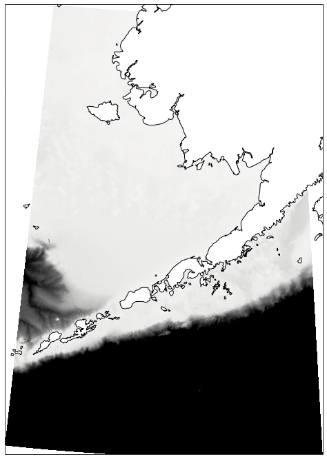
shaded bathymetry data (instead of an image or a solid color for water)
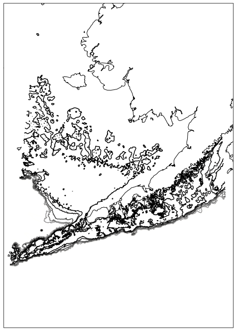
contours at regular or irregular intervals

Plotting Packages that make this convenient

Cartopy and Matplotlib
GMT

Data Sources

examples rely on erddap or builtin datasets
easy to extend to other erddap hosted bathymetry, or netcdf files just by changing source data in the xarray calls

Cartopy + Matplotlib + erddap/xarray¶

The following example relys on cartopy+matplotlib

Using Matplotlib (a very common plotting library) and cartopy to create plots. If you are familiar with matplotlib syntax and arguments, this is a small learning curve. Plots can be tweaked and the package dependencies are usually pretty stable.

The data is hosted on an erddap server, no special API is needed to download a gridded dataset via opendap protocal

import xarray as xa
import matplotlib.pyplot as plt

import cartopy.crs as ccrs
import cartopy.feature as cfeature
from cartopy.mpl.ticker import LongitudeFormatter, LatitudeFormatter

import cmocean #ocean colormaps

extent=[-170, -155, 50, 63]

erddap_grid = xa.open_dataset('https://coastwatch.pfeg.noaa.gov/erddap/griddap/usgsCeSS111')

#given your extent of interst, subset the data to make the contouring quicker... no need to do this globally if you only want the Bering Sea
erddap_grid_sub = erddap_grid.sel(latitude=slice(extent[3],extent[2]),longitude=slice(extent[0],extent[1]))

def make_map(projection=ccrs.PlateCarree()):
    fig, ax = plt.subplots(figsize=(12,12),
                           subplot_kw=dict(projection=projection))
    if projection == ccrs.PlateCarree():
        gl = ax.gridlines(draw_labels=True)
        gl.xlabels_top = gl.ylabels_right = False
        gl.xformatter = LONGITUDE_FORMATTER
        gl.yformatter = LATITUDE_FORMATTER
    return fig, ax

#some basic map projection manipulation and transformation is involved here
# datasets can be large and take time to render so don't go to crazy

with_topo = True

projection=ccrs.LambertConformal(central_longitude=-160.0)
transformation=ccrs.PlateCarree()


fig,ax = make_map(projection=projection)

if with_topo:
    ax.pcolormesh(erddap_grid_sub.longitude, erddap_grid_sub.latitude, 
                erddap_grid_sub.topo, cmap=cmocean.cm.gray,
                vmin=-3000,vmax=100,
                transform=transformation)

ax.add_feature(cfeature.NaturalEarthFeature('physical','coastline','10m',edgecolor='k',facecolor='w'))

ax.set_extent(extent)
plt.show()

../../../_images/Map_contours_examples_5_0.png

#some basic map projection manipulation and transformation is involved here
# datasets can be large and take time to render so don't go to crazy

with_topo = True

projection=ccrs.LambertConformal(central_longitude=-160.0)
transformation=ccrs.PlateCarree()


fig,ax = make_map(projection=projection)

if with_topo:
    ax.contour(erddap_grid_sub.longitude, erddap_grid_sub.latitude, 
                erddap_grid_sub.topo, cmap=cmocean.cm.gray_r,
                levels=[-1500,-1000,-750,-500,-250,-150,-70],
                transform=transformation)

ax.add_feature(cfeature.NaturalEarthFeature('physical','coastline','10m',edgecolor='k',facecolor='w'))

ax.set_extent(extent)
plt.show()

../../../_images/Map_contours_examples_6_0.png

Other Tasks that can easily be done

contour fill the ocean or change colors
add labels to contours
use coarser datasets for smoother contours

GMT¶

The following example is using GMT (an actively developed pythonic port of GMT 6) with installation instructions available at https://www.pygmt.org/latest/.

Personally, there is a lot of strengths to using this well developed package, not limited to the creation of very professional looking plots.- but it can occasionally be hard to install / keep up to date / follow along with examples and sometimes you have to “port” examples or details from pure GMT syntax to pyGMT syntax with little more than the pure GMT references.

I recomend using an environment manager (like whats built in to Conda) to manage pygmt and its dependancies

import pygmt

grid = pygmt.datasets.load_earth_relief(resolution="01m", region=extent) #datasets here can be found in the documentation... many are SRTM derived at high res and will be downloaded to start

fig = pygmt.Figure()
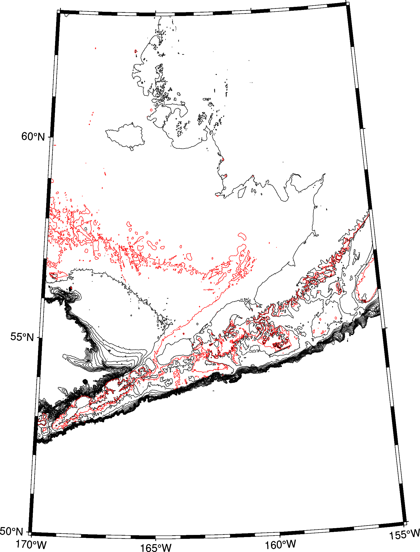
#fixed interval grids with a secondary color for a isobath of interest
# in this case countour 0,100,200...1500 in black and 70m in red and don't label anything
fig.grdcontour(annotation=None,
               interval=100,
               grid=grid,
               limit=[-1500, 0],
               projection="L-165/35/33/45/12c",
               frame=True,)
fig.grdcontour(annotation=None,
               interval=70,
               grid=grid,
               limit=[-100, -1],
               projection="L-165/35/33/45/12c",
               pen="red",
               frame=True,)
fig.show()

../../../_images/Map_contours_examples_11_0.png

Other Tasks that can easily be done

fill in land or contour fill the ocean
add labels to contours
irregular contours
usage of other gridded datasets including those from netcdf files (not just the builtin datasets)

EcoSystems Fisheries-Oceanograpy Coordinated Investigations (EcoFOCI)

Two ways to use bathymetric datasets to generate bathymetry contours in a plot¶

Cartopy + Matplotlib + erddap/xarray¶

GMT¶